PeN-model
"PeN-model"is the acronym for a numerical model of the atmosphere that was developed at IMAU (Utrecht University) for education purposes for the courses, Dynamical Meteorology, Climate and the Hydrological Cycle and Simulation of Oceans, Atmospheres and Climate. Pe stands for "primitive equations" and N stands for N layers. A 3D version of the model with N=36 and a 2D version of the model with N=200 are "operational". The 3D version is used to study the life cycles of baroclinic waves (cyclones and anticyclones) in middle latitudes, while the 2D version is used to study the interaction between adiabatic dynamics and diabatic processes, such as absorption and emission of radiation and latent heat release, in the General Circulation. This version can be used to understand the subtropical jet, the Hadley circulation and the polar winter stratospheric vortex. The 2D version of the model includes parametrizations of planetary wave drag and the water cycle. The water cycle and wave drag can easily be switched on or off. On this page two simulations with the 2D model are described.
2D-SIMULATION OF THE ZONAL MEAN STATE OF THE ATMOSPHERE: zero obliquity
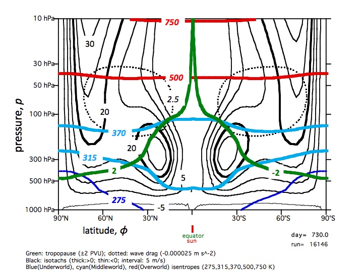
Several simulations with the 2D version of the model were performed with zero obliquity, sometimes referred to as "permanent equinox simulations". Run 1f represents a permanent equinox simulation which includes all the important physical processes, except absorption Solar radiation by ozone. It includes dry convective adjustment, planetary wave drag and water cycle. The most important elements of the water cycle are evaporation, which is largest in the (sub)tropics, and condensation, which is largest over the Inter Tropical Convergence Zone (ITCZ). The upper (first) panel on the right shows the zonal wind (black contours, labeled in units of m/s), the potential temperature (red, cyan and blue lines, labeled in units of K) and the dynamical tropopause (green, labeled in PVU) after 730 days (2 years) of simulation. At t=0 the atmosphere is isothermal l (at 290 K) and in rest. Within the dotted lines the westward force per unit mass, due wave-drag, is greater than 0.0025 m/s^2. Wave drag is imposed only if the zonal wind is eastward both locally and at all levels below. This is based on the theoretical idea that planetary waves cannot propagate upward through the atmosphere if the wind is westward. Blue lines indicate "Underworld" isentropes. The cyan lines indicate "Middleworld" isentropes. Red lines indicate "Overworld" isentropes. This terminology was introduced by N. Shaw in 1931and refined by B. Hoskins in 1991. Middleworld isentropes intersect the dynamical tropopause. The Middleworld is a very important layer in the atmosphere, because it contains the subtropical jets. It is also the layer where the stratosphere (in the extratropics) stands in adibatic contact with the troposphere (in the tropics). It contains more mass per square metre in the tropics than in the extratropics. The atmosphere is close to a steady state after 2 years. Subtropical jets have formed, with a maximum wind speed of 27 m/s at 250 hPa and ±25° latitude. The stratospheric polar night jet, centred at ±65° latitude, is formed much more slowly than the subtropical jets, which are connected to the Hadly circulation. This circulation is driven mainly by latent heat release between 900 hPa and 200 hPa above the ITCZ at the equator.
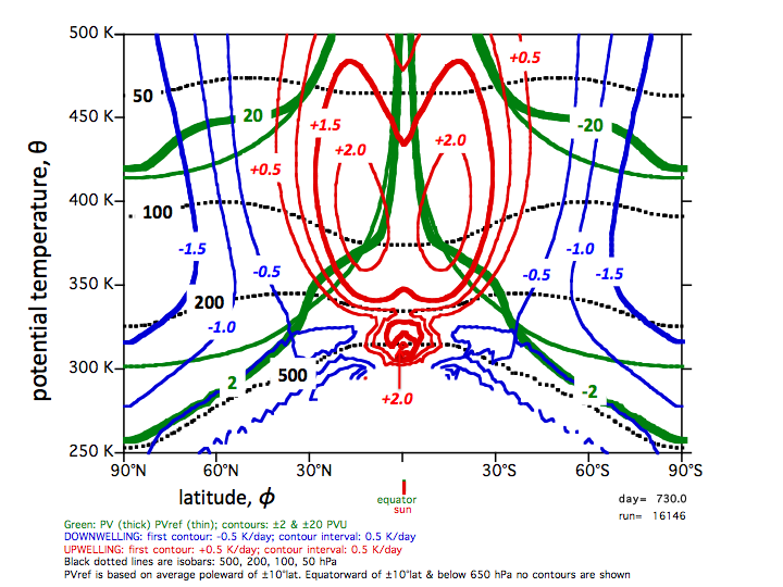
The second panel at the right shows the cross-isentropic flow and the potential vorticity, both in the reference state of rest (thin green lines) and in the actual state (thick green line). The dynamical tropopause corresponds to the lowest thick green isopleth of PV, labeled ±2 PVU. Lines of equal pressure are indicated by the dotted black lines, labeled in hPa. Cross-isentropic flow is upward (red contours) in the tropics and downward (blue contours) in the extratropics, in agreement with reality. You can watch the corresponding animation by clicking on the icon "Run1f" (or m4v format"Run1f" for ipad).
2D-SIMULATION OF THE ZONAL MEAN STATE OF THE ATMOSPHERE: seasonal cycle
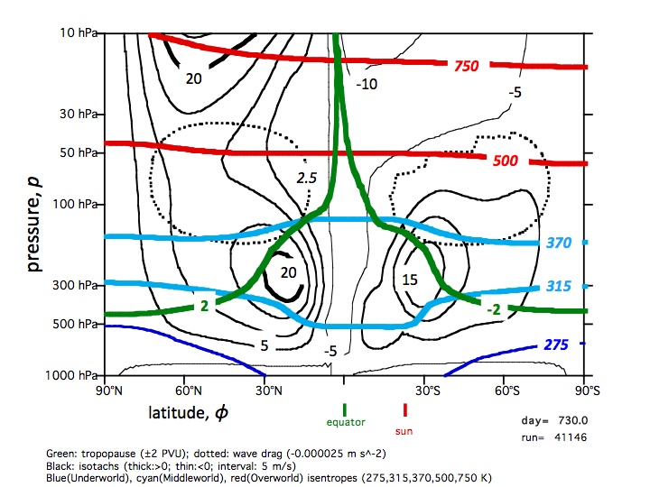
The third and fourth panels on the right display output of the "best" simulation of the zonal mean state of the atmosphere, including its seasonal cycle. The obliquity is set to 23.45°. Again, the model is initialized with an isothermal (290 K) atmosphere in rest. A realistic simulation is obtained only if wave drag is included in the model. The third panel indicates that the winter subtropical jet at 20°N-30°N is stronger than the summer subtropical jet (at 30°S), in agreement with observations. The tropopause is approximately at the right height. The upward bulge of the 370 K isentrope in the tropics, which is also seen in run 1f, is an indication of the presence of a tropical cold layer at about 100 hPa, which agrees with reality. You can watch the corresponding animation by clicking on the icon "Run4a" (or m4v format"Run4a" for ipad).
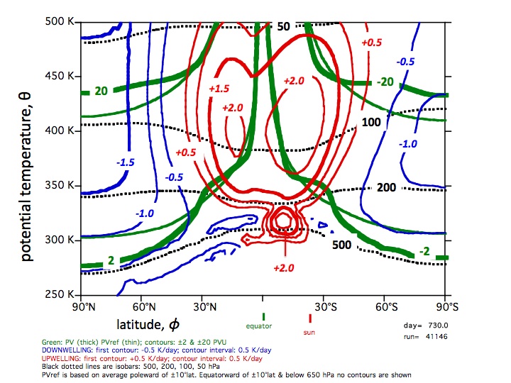
The fourth panel shows the cross-isentropic flow on January 1 of year 3 of the same simulation, as a function of latitude and potential temperature. Lines of equal pressure are indicated by the dotted black lines, labeled in hPa. Cross-isentropic flow is upward (red contours) in the tropics and downward (blue contours) in the extratropics, in agreement with reality. This is not a trivial matter. If only radiation were to determine the cross-isentropic or diabatic circulation, this circulation would consist of only one cell: upward in the summer and downward in the winter. Radiation flux divergence and the diabatic circulation together determine the vertical position of the dynamical tropopause, which is defined as the ±2 PVU isopleth of the potential vorticity (the lower thick green contour).
CONCLUSION ON 2D-SIMULATIONS
The 2D version of the PeN model reproduces many realistic characteristics of the zonal mean general circulation of the atmosphere. This can be verified by watching the movies, which show how the model state, shown in the figures, is reached, after the model is initialized with an isothermal atmosphere (290 K) in rest on January 1 of year 1.
A paper (see pdf) on this topic will be published in Tellus in November 2014 (see publications). Here is the pdf of a seminar held at Reading University on 10 November 2014: pdf
Results of baroclinic life cycle experiments with the 3D version of the PeN model are described in chapter 10 of the lecture notes on Atmospheric Dynamics: link.
How did the atmosphere reach this steady state? Watch this movie: Run1f
(or m4v format"Run1f" for ipad)
How did the atmosphere reach this steady state? Watch this movie: Run1f
How did the atmosphere reach this state? Watch this movie: Run4a
(or m4v format"Run4a" for ipad).
How did the atmosphere reach this state? Watch this movie: Run4a
Background material
LECTURE NOTES
The PeN-model is described in chapters 10 and 12 of the lecture notes on Atmospheric Dynamics: link
See also the page describing the project "Circulation & global change": link
Acknowledgement
I wish to thank Koen Manders, Niels Zweers and Roos de Wit for help in developing and debugging the numerical model and for stimulating scientific input in the early stages of this research project, Yvonne Hinssen and Theo Opsteegh for useful discussions on potential vorticity inversion, Bruce Denby for his large contribution in developing the computer graphics, the students of my course on climate and the water cycle for useful suggestions on incorporating and validating the parametrizations associated with the water cycle, Marcel Portanger for advice and help on computer problems and, finally, all my colleagues at IMAU for allowing me to work on such a large and time-consuming project.