User's guide Mondriaan version 4.2.1
This page is continuously being improved and updated; therefore, a more recent version may be obtained online. This offline version is bundled with the software for your convenience.
How to download and install Mondriaan
Download the latest version from the Mondriaan software homepage. Uncompress with, e.g.,
% tar xzvf mondriaan4.tar.gz
(Here, '%' is the prompt of your operating system.)
This will create a directory Mondriaan4
which contains all the files of the Mondriaan package.
Important files are:
README, which tells you about copyright and how to cite the work.COPYING, the GNU General Public License (GNU GPL).COPYING.LESSER, the GNU Lesser General Public License (GNU LGPL), which is an addition to GNU GPL, making its use more liberal.mondriaan.mk, which contains the Mondriaan compilation options.
How to compile and test Mondriaan
Go inside the directory Mondriaan4 and type
% make
This will compile the Mondriaan library, the MondriaanOpt library and
tools included with the Mondriaan library.
After compilation the include files are located in Mondriaan4/src/include,
the compiled library in Mondriaan4/src/lib,
and the stand-alone Mondriaan tools in Mondriaan4/tools.
An example of how to use the Mondriaan library in your own
program is provided by Mondriaan4/docs/example.c and
Mondriaan4/tools/Mondriaan.c.
For more information about MATLAB usage, please see the Mondriaan MATLAB guide.
To enable MATLAB support for Mondriaan and MondriaanOpt, edit the file
mondriaan.mk and change the line containing the variable
MATLABHOMEDIR to your current MATLAB install directory and
remove the '#' in front of the line to uncomment it.
The variable MEXSUFFIX should be set to the appropriate
extension for your platform, as specified on the Mathworks site.
This should be done before compiling Mondriaan.
Similarly, to enable PaToH support (the PaToH library can be found
here),
edit mondriaan.mk to change the line containing the PATOHHOMEDIR variable, as detailed above.
For each function of the core Mondriaan program,
we have written a small (undocumented) test, which checks those functions
for proper behaviour. The unit tests have been tried successfully on two
architectures: Linux and Mac Os X. If one or more of the tests fails,
please try to identify the relevant error message, and inform me
(R . H . Bisseling @ NOSPAM uu . nl ) about the problem. I will try to help you
solve it. The tests called can be found in the script runtest
residing in the tests/ subdirectory.
To compile and run all 109 unit tests, type
% make test
Timers
The compile option -DTIME causes the CPU time used by Mondriaan
for the matrix distribution to be printed, and also the time for the vector
distribution. This timer has a relatively low (guaranteed) accuracy, and
it is in danger of clock wraparound.
The compile option -DUNIX tells Mondriaan
you are using a UNIX system.
Together with -DTIME this also causes the elapsed (wall clock)
time to be printed, which is an upper bound on the CPU time.
Usually the timer accuracy is higher, and there is no danger of clock
wraparound. This is the best timer if you are the single user of the system.
Levels of verbosity
Mondriaan writes the output distributions to file.
It can also generate useful statistics about the partitioning
to the standard output stream stdout (or the screen).
There are three levels of verbosity: silent, standard, and verbose.
The silent mode is useful when running the unit tests by
make test. (If these are not done silently,
the OKs are obscured.)
The silent mode may also be useful if (parts of) Mondriaan are used as library
functions.
The verbose mode is useful when debugging, or trying to understand
a particular run in detail.
The standard mode generates 1-2 pages of output, and
is aimed at easy digestion.
You can change the verbosity level by commenting and uncommenting
the appropriate CFLAGS lines in mondriaan.mk.
Using the flag -DINFO generates standard output,
and using the flags -DINFO -DINFO2 generates verbose output.
How to run Mondriaan
Go inside the directory Mondriaan4 and type
% cd tools% ./Mondriaan ../tests/arc130.mtx 8 0.03
if you want to partition the arc130.mtx matrix (Matrix Market file format)
for 8 processors with at most 3% load imbalance. The matrix should be the full
relative path; in the above example output is saved in the Mondriaan tests folder (../tests/).
Mondriaan may also be used to partition matrices provided via the standard
input, e.g., by using piping:
% cat ../tests/arc130.mtx | ./Mondriaan - 8 0.03
to obtain the same result as with the previous method, with one difference:
results are written in the current (tools) directory.
For integration with already existing software you may have, without resorting to writing and reading files (or pipes),
look at the how to use Mondriaan as a library section of this guide.
Output
The main Mondriaan tool yields, after a successful run on an input matrix,
various output files. All possible output files are described below. Typically,
the output filenames are that of the input matrix filename, appended with a small
descriptor and usually the number of parts x Mondriaan was requested to
construct.
Distributed matrix (-Px)
The Mondriaan program writes the distributed matrix to a file called
input-Px,
where input is the name of the input matrix, or stdin if the
matrix was read from the standard input, and x is the number of processors
used in the distribution.
We use an adapted Matrix Market format, with this structure:
%%MatrixMarket distributed-matrix coordinate real general ( this should be 0 )
m n nnz P
Pstart[0]
...
...
...
Pstart[P]( this should be nnz )
A.i[0] A.j[0] A.value[0]
...
...
...
A.i[nnz-1] A.j[nnz-1] A.value[nnz-1]
Here, Pstart[k] points to the start of the nonzeroes
of processor k.
Processor indices (-Ix)
The Mondriaan program also writes the processor indices of each
nonzero to the Matrix Market file input-Ix where the value of each
nonzero is replaced by the processor index to which the nonzero has been assigned.
The order of the nonzeroes is exactly that of the distributed matrix (-Px).
Row and column permutations (-rowx, -colx)
Mondriaan writes the row and column permutations determined by the
Mondriaan algorithm (set by the Permute option) to input-rowx
and input-colx. The goal of these permutations is to bring the input
matrix A into (doubly) Separated Block Diagonal (SBD) or Bordered Block
Diagonal (BBD) form, after applying the found permutations. This can have many
possible applications, including, but not limited to, cache-oblivious sparse
matrix vector multiplication (SBD form) or minimising fill-in in sparse LU
decomposition (BBD form). These files are not written if the Permute
option is set to none.
Reordered matrix (-reor-Px)
Mondriaan also directly writes the permuted matrix PAQ to
file, where the permutation matrix P corresponds to the row permutation
determined by the Mondriaan algorithm, as described in the previous paragraph.
The permutation matrix Q is similarly inferred from the column
permutation. This file is not written if the Permute option is set
to none.
Separator boundary indices & hierarchy
(-rowblocksx, -colblocksx)
These two files store two column-vectors each. The first column-vector relates to the separator boundary indices, the second to the separator hierarchy structure. The vectors are stored next to each other, so that each file has two columns of integers and m, resp, n rows. Each will be explained in turn.

The (doubly) separated block diagonal and bordered block diagonal forms
each identify groups of nonzeroes, the separators, which serve as
connectors between two parts resulting from a single bipartition. In the
reordered matrix described above, these groups appear as relatively dense
and usually small strips of consecutive rows and columns; the separator
blocks. The indices where these blocks start and end in the reordered
matrix are given in these two files; this is done by consecutively listing
the start index and end index of each block, both separator and
non-separator, as they occur in the row and column direction. These files
are not written if the Permute option is set to none.
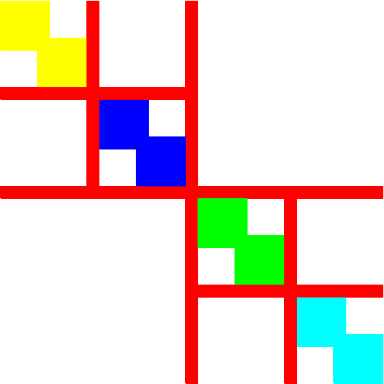
A more detailed explanation follows from the (idealised) Figures 1 and 2. The first shows a reordering corresponding to a single bipartition, clearly yielding four row and column indices indicating the start and end of the differently coloured partitions. This can occur recursively as shown in the second figure; there, each non-red partition is an instance of Figure 1, resulting in 16 row and column indices indicating the separators for the eight partitions. Assuming each non-separator block is two-by-two (x=2 in Figure 3), and the separator blocks are only one row and one column thick ( ~x=1), then the row and column boundary indices would equal (0,2,3,5,6,8,9,...,21,23). These two arrays are stored as a column vector in each file.
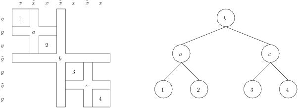
The second column in each file describes the separator hierarchy. As Mondriaan follows a bipartitioning scheme, the separator block from the very first bipartitioning corresponds to the separator blocks spanning the entire matrix. As bipartitioning is then called recursively, the separator blocks span only a subpart of the reordered matrix, and can be viewed as a child of the largest separator blocks; in this way a binary tree of separator blocks can be defined. See Figure 3 for clarification.
Each row of the rowblocks and columnblocks file
corresponds to the start of a block (excluding the very last row which
always equals m+1, resp., n+1, where m by n is the matrix size).
Integers from 1 to m or 1 to n thus indicate blocks, and each separator
block can point to its parent separator block by using these indices.
This is exactly what is stored in the second column, where each
non-separator block points to the separator block constructed in the
same bipartitioning, and all separator blocks point to their direct
parent separator block, as in Figure 3. The root separator, the one
constructed in the very first bipartitioning, has no parent and
therefore points to the non-existing index zero. Continuing the
example, both the row and column hierarchies would be given by the
array (2,4,2,8,6,4,6,0,10,12,10,8,14,12,14).
The rowblocks file in this instance would then look as follows (only
partially shown):
0 2

2 4

3 2

5 8

...

21 14

23
Input/output vector distributions (-ux, -vx)
The program writes the processor numbers of the vector components
to the files called input-ux and input-vx,
where input is the name of the input matrix
and x is the number of processors used in the distribution.
The vectors u and v are the output and input vectors
of the sparse matrix-vector multiplication u=A*v.
In I/O files, all indices (i,j) for matrix entries a(i,j) and vector components u(i) and v(j) start numbering from 1, following the Matrix Market conventions. In I/O, the processors are numbered 1 to P. Internally, the indices are converted to the standard C-numbering starting from 0.
Cartesian submatrices (-Cx)
The program writes the row index sets I(q)
and column index sets J(q) of the Cartesian submatrix I(q) x J(q)
for the processors q=1,...,P to the file called input-Cx,
where input is the name of the input matrix
and x is the number of processors used in the distribution.
This file is additional information, useful e.g. for visualisation,
and you may not need it.
Statistics on standard output
Provided the library is compiled with the -DINFO or -DINFO2 option,
the program prints plenty of useful statistics to standard output.
The communication volume is given for the two phases
of the matrix-vector multiplication separately:
the volume for v (first communication phase)
and the volume for u (second communication phase).
The bottom line is the communication cost
which is defined as the sum of the costs of the two phases.
The cost of a phase is the maximum of the number of data words
sent and the number of data words received, over all processors.
This metric is also called the BSP cost; it is the cost
metric of the Bulk Synchronous Parallel model.
Graphical output
In the tools/ subdirectory the program MondriaanPlot
can be used to get insight in the Mondriaan partitioning algorithm.
This program creates a series of Truevision TGA image files named
img0000.tga, img0001.tga, ..., up to the number of
processors over which the matrix is divided.
To use this program, issue
% cd tools% ./MondriaanPlot ../tests/arc130.mtx 8 0.03
If you have mencoder installed, you can use the MondriaanMovie
script to generate a small movie of the partitioning process:
% ./MondriaanMovie ../tests/arc130.mtx 8 0.03
This will create ../tests/arc130.mtx.avi.
If you have imagemagick installed (or if the convert command is
otherwise available), you can use MondriaanGIF to create an animated
GIF of the partitioning process:
% ./MondriaanGIF ../tests/arc130.mtx 8 0.03
This will create ../tests/arc130.mtx.gif.
When creating images with MondriaanPlot, also an SVG file is generated.
Just as the .tga files, the .svg file also contains a visualisation of the partitioning.
In the above examples, the svg file created will be ../tests/arc130.mtx-8.svg.
Program options
The Mondriaan options can be set in the
Mondriaan.defaults file. If no such file exists, it is created
at run time. Afterwards, this file can be edited for further runs.
The default values of the options are given below in boldface.
It is possible to overrule the defaults from the command line,
e.g. by typing
% ./Mondriaan ../tests/arc130.mtx 8 0.03 -SplitStrategy=onedimrow
you can force Mondriaan to split the matrix in one dimension only, namely by rows.
Nonnumerical options
The nonnumerical options are used to choose partitioning methods. You may need to change them from the defaults to explore different partitioning methods.
Output options
Numerical options
The numerical options are often used to optimise given partitioning methods.
Setting values such as NrRestarts,
MaxNrLoops, or
MaxNrNoGainMoves to a higher number, often results in better quality
of the partitioning solution, at the expense of increased run-time.
How to use Mondriaan as a library
After successful compilation (using make),
all relevant header files are exported to the src/include directory,
and a static library is available in the src/lib directory.
To illustrate the use of Mondriaan we provide a small example program together with this guide. This example can be compiled (provided the Mondriaan library was successfully built) by executing
% gcc -DGAINBUCKET_ARRAY example.c -I../src/include -L../src/lib -lMondriaan4 -lm
in the docs/ directory which will generate the executable a.out.
More advanced use of the library is illustrated in tools/Mondriaan.c.
Mondriaan uses a triplet-based datastructure (the Matrix Market format) to store sparse matrices;
that is, for each nonzero, its row- and column-index are stored, as well as its numerical value (in general).
The exact representation is detailed in src/SparseMatrix.c/.h; and to successfully interface,
your sparse matrix scheme has to be translated into this format.
Since the Compressed Row Storage (CRS), or alternatively known as Compressed Sparse Row (CSR), is a more prevailing standard,
SparseMatrix comes with a translation function specifically for that datastructure: CRSSparseMatrixInit.
It takes as input an uninitialised Mondriaan SparseMatrix struct, the matrix dimensions and number of nonzeroes, and
the CRS datastructure arrays. The base parameter automatically translates from, e.g., 1-based arrays (base=1) as
they may appear in for example Fortran, to 0-based arrays as used in Mondriaan.
Next is setting any options for Mondriaan. Recommended is to use an options file, storing all the defaults tuned to your application (e.g. as provided by tools/Mondriaan.defaults).
These defaults can be read from file and stored in the Mondriaan Options struct by using the function SetOptionsFromFile;
see src/Options.c/.h.
Once both the sparse matrix and the options are ready the main Mondriaan distribution function, DistributeMatrixMondriaan, can be used.
This function takes as parameters the sparse matrix struct, the number of processors, the load imbalance parameter, and the options struct.
The callback function is for advanced use, and is usually kept a NULL pointer (an example of using the callback is given in tools/MondriaanPlot.c). This function is a blocking call.
After partitioning, all relevant information can be extracted from the SparseMatrix struct (see the source code for details).
The struct can be freed by calling MMDeleteSparseMatrix.
Interfacing with non-C code is best achieved by writing a custom interface between your code and Mondriaan, using extern "C"-style additions when, e.g., interfacing between C++ and C; or using any other specific translation required (e.g., writing all parameters as pointers (Fortran), using jni (Java), etc.).
As an example, the MATLAB interface is given in tools/MatlabMondriaan.c.
Profiling Mondriaan
To profile the Mondriaan library for various configurations, please use
the Profile program and RunProfiler script both included
in the tools/ directory.
Entering the tools/ directory and executing
% ./Profile 8 0.03 10 a.mtx b.mtx c.mtx > out.tex
partitions the matrices a.mtx, b.mtx, and c.mtx
among 8 processors with at most 3% imbalance, taking the average over 10
runs with a different random seed.
The results are written, via stdout, to the LaTeX file out.tex
which then contains a table with the averaged results of the partitioning
process.
For code developers
If you develop new code to add to Mondriaan, you probably would like to add possibilities to use your code through a new option. In that case you need to adjust a few files:
src/Options.h: you should add the option and its possible values.src/Options.c: you should make a choice for the default value and set it in the functionSetDefaultOptions. If the option is a numerical option, you should check its range in the functionSetDefaultOptions. Finally, you should add the option and all its possible values as an if-statement in the functionSetOption.- subdirectory
tests: it may happen that adding the options will break a few unit tests, in particular those connected to functionsGetParameters,SetDefaultOptions,SetOption. This is quite harmless, and easy to repair.
More information
All functions of Mondriaan have extensive documentation in the source code (.c files).
Please have a look there for more details.
References
[1]
Cache-oblivious sparse matrix-vector multiplication by using sparse matrix partitioning methods,
A. N. Yzelman and Rob H. Bisseling, SIAM Journal of Scientific Computation, Vol. 31, Issue 4, pp. 3128-3154 (2009).
[2]
Two-dimensional cache-oblivious sparse matrix-vector multiplication,
A. N. Yzelman and Rob H. Bisseling, Parallel Computing, Vol. 37, Issue 12, pp. 806-819 (2011).
[3]
A medium-grain method for fast 2D bipartitioning of sparse matrices,
Daniël M. Pelt and Rob H. Bisseling, Proceedings IEEE International Parallel
and Distributed Processing Symposium 2014, IEEE Press, pp. 529-539.
[4]
A new metric enabling an exact hypergraph model for the communication volume in distributed-memory parallel applications
O. Fortmeier, H. M. Bücker, B. O. Fagginger Auer, R. H. Bisseling, Parallel Computing, Vol. 39, Issue 8, pp. 319-335 (2013).
[5]
A Fine-Grain Hypergraph Model for 2D Decomposition of Sparse Matrices
Ümit V. Çatalyürek and Cevdet Aykanat, IPDPS 2001, p. 118 (2001).
[6]
Communication balancing in parallel sparse matrix-vector multiplication
Rob H. Bisseling and Wouter Meesen, ETNA, pp. 47-65 (2005).
[7]
Two-Dimensional Approaches to Sparse Matrix Partitioning
Rob H. Bisseling, Bas O. Fagginger Auer, A. N. Yzelman, Tristan van Leeuwen and Ümit V. Çatalyürek,
Chapter 12 of Combinatorial Scientific Computing, Chapman and Hall/CRC, pp. 321-349 (2012).
Last updated: December 18, 2020.
June 9, 2009 by Rob Bisseling,
December 2, 2010 by Bas Fagginger Auer,
December 10, 2010 by A. N. Yzelman,
March 27, 2012 by Bas Fagginger Auer,
April 18, 2013 by Daniël M. Pelt,
August 29, 2013 by Rob Bisseling and Bas Fagginger Auer,
October 27, 2016 by Marco van Oort,
September 7, 2017 by Marco van Oort.
To
the Mondriaan package home page.
