Goal:

Study the CO budget. Compare simulated CO values to CO measurements. Analyze the contribution of different CO sources to the CO levels in the atmosphere.

Introduction

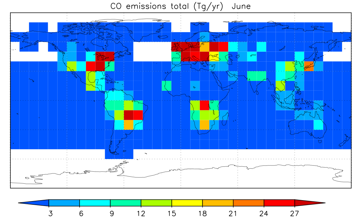
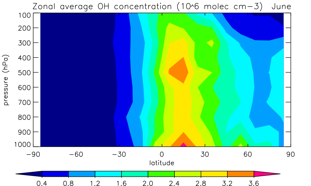
Tropospheric CO strongly influences the oxidation efficiency of our atmosphere. More than half the hydroxyl radical (OH) removal from the atmosphere is caused by the reaction with OH. This reaction is also the dominant sink for CO as surface deposition and other reaction pathways are negligible. Biomass burning and fossil fuel combustion are main anthropogenic CO sources that account for about 40% of the global source.

Source Category	CO emission (Tg/year)
Energy use	540
Anthropogenic biomass burning	400
Wildfires	30
Vegetation	100
Oxidation of natural CH4	250
Oxidation of anthropogenic CH4	595
Oxidation of natural NMHC	325
Oxidation of anthropogenic NMHC	120
Oceans	40
Total	2400

Table 1: Emissions of CO expressed in teragram (Tg) per year, 1 Tg = 10¹² g.

Increasing CO as a consequence of anthropogenic emissions in the past century has likely contributed to a global depletion of OH and thus a reduction of the oxidation efficiency of the atmosphere. On the other hand, the recent trend reversal of CO, possibly due to a moderation of anthropogenic emissions, may have contributed to a partial recovery of OH levels. Global observations and the quantification of CO changes and its budget are of utmost importance to monitor the state of our atmosphere.

Although the global CO burden of the atmosphere is fairly well known, the estimates of source categories are highly uncertain. Most of the emission estimates have uncertainty ranges of about 50%. For example, the CO yield from non-methane hydrocarbon (NMHC) oxidation in the atmosphere is poorly known. Large quantities of natural NMHC are emitted as isoprene and monoterpenes. Both the emissions of these gases and their reaction products are poorly quantified. If removal of soluble or aerosol forming NMHC reaction intermediates would be important, this would substantially limit the amount of CO released from these compounds. Models can help quantifying these processes by integration of the growing knowledge about sources, transport and chemical mechanisms, and through comparisons with observations.

The lifetime of CO varies considerably in the atmosphere. In the high latitude winter it is very long (>0.5 year) because the OH radical concentrations are very low. At low altitudes in the tropics, where both radiation and water vapor abundance promote OH radical formation, the CO lifetime drops to values less than a month. At mid-latitudes the seasonal cycle is characterized by CO buildup in winter and depletion in summer. On the one hand, CO lives long enough to be transported over considerable distances. On the other hand, its lifetime is short enough that it can be present in the background atmosphere in rather small concentrations.

Exercise 5: The CO distribution

In this exercise, the CO distribution will be modeled (in a simplified way). CO is treated as a tracer, which is

1. emitted at the surface by monthly varying emission fields (see figure 1)
2. produced from oxidation of methane: CH4 + OH ---> (intermediates) ---> CO
3. destroyed by OH: CO + OH ---> CO2 + H. (figure 2 shows OH distributions)

Figure 2: Zonal average OH concentrations in June (left) and December (right).

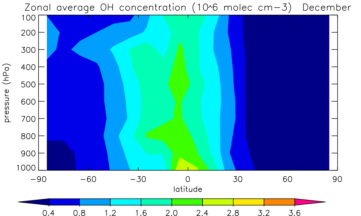CO lives about two months, so a spin-up time of 5 months is used to initiate the model. The pre-calculated OH fields are stored on disk and are used in the input file by the commands:

• CHEMISTRY (to model CO destruction by OH)
• EMISSION OH (to model CO production by CH4 + OH)

Precooked emission files are present:

• Run MOGUNTIA with input file co1.in to spin up the model
• Run MOGUNTIA with input file co2.in to generate output

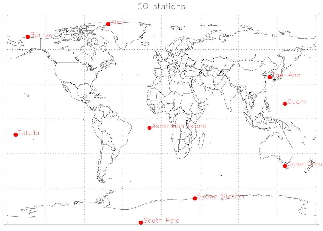
CO is measured mainly by ground based stations. In this exercise, the CO simulations are compared to measurements at the following stations (see map on the right for locations:

Alert (82N, 62W) Ascension Island (8S, 14W) Barrow (71N, 156W) Cape Grim (41S, 144E) Guam (13N, 144E) Tutuila (14S , 170W) South Pole (90S, 24W) Syowa Station (69S, 39E) Tae-ahn (36N, 126E)

Concentration of CO are normally expressed as ppbv, which corresponds to a mixing ratio of 10^-9. Due to variability in emissions and variability in the transport to the measurement sites, large year-to-year variability in the CO concentrations is observed for most sites. Only remote stations show a regular pattern.

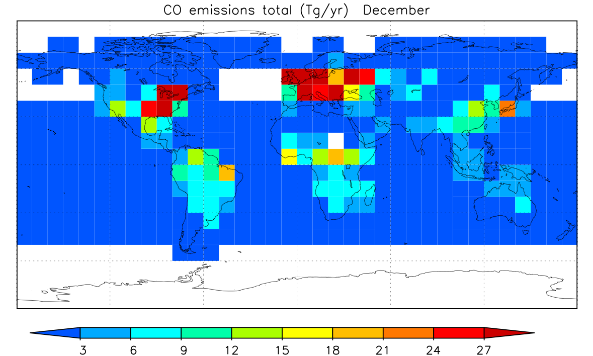
Since the MOGUNTIA model is climatological and uses only one year of meteorological data (1987), variability in transport cannot be simulated. Also, variability is emissions is not simulated, since the quantification of emissions is quite difficult. For instance, biomass burning has a large year-to-year variability (e.g. Indonesian fires).

• Compare the simulated CO levels to the measurements at the stations
• What stations compare well, what stations compare not so well? Differentiate between NH, SH and equatorial stations.
• Explain and compare the seasonal cycles.
• What can be the cause for the observed (and simulated?) double peak in some seasonal cycles?
• Discuss possible causes of poor simulation (look at concentration gradients near the stations, discuss systematic higher/lower concentrations in terms of possible missing/overestimated sources)

Exercise 6, the budget of CO

In order to study the contribution of the various sources to the CO levels at the stations, we investigate first how much of the CO is generated by methane oxidation. Precooked input files, in which the surface CO emissions are switched off can be used:.

• Run MOGUNTIA with input file co_methane1.in to spin up the model
• Run MOGUNTIA with input file co_methane2.in to generate output.

Analysis of the output

• Explain the global CO distribution from the methane oxidation.
• Can the seasonal cycle of CO be explained by the methane oxidation source? Why?

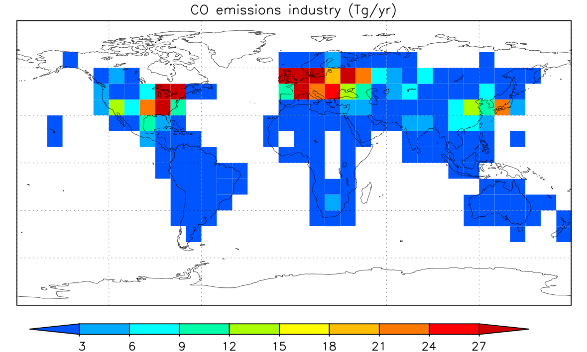
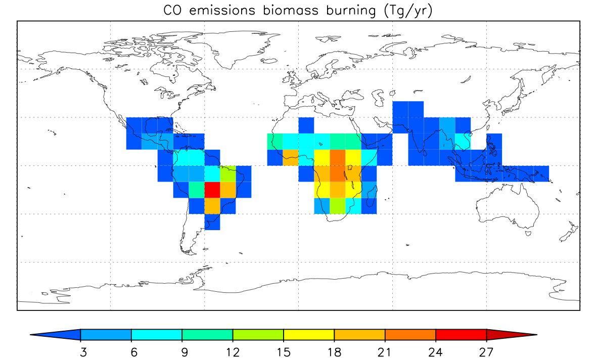
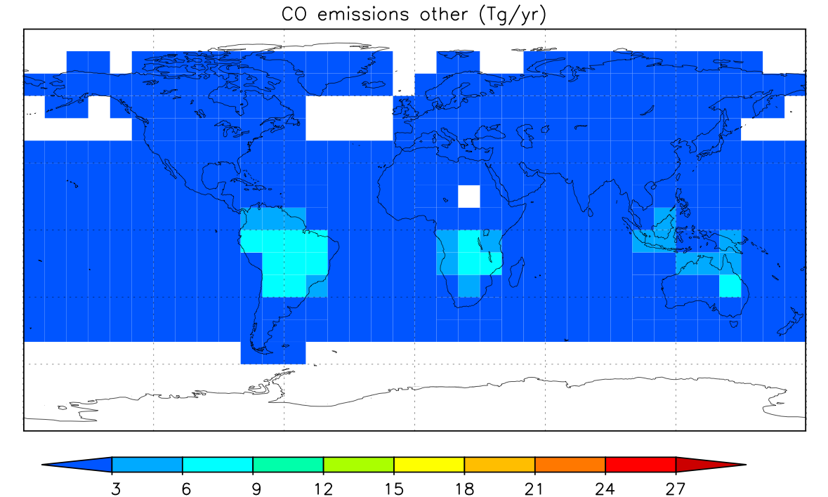
The input files co_budget1.in and co_budget2.in describe a simulation with industrial emissions as the only CO source. Run MOGUNTIA with these input files. Then run MOGUNTIA also with other sources (see figure 3) switched on. For example: to activate only the biomass sources, the input file should look like:

TITLE co_budget_bmb (remember to change the title to generate separate output files)

NAME co

MOLMASS 28.0

START_CONCENTRATION 0.0/PREVIOUS (depending on spin up or output generation)

EMISSION FILE co_emissions_bmb.dat

(other emission lines deactivated by a starting blanc)

  ........etc......

Figure 3: CO emissions from industry, biomass burning and other surface sources.

• Discuss the contribution of the various sources to the concentrations measured at the stations.
• Which source category should be higher or lower to improve the comparison?