Remember that estimation of ??? is equivalent to an estimation of OH.
- How consistent is the derived removal rate over longer periods?
Exercise 7: Determine the rate constant for MCF + OH
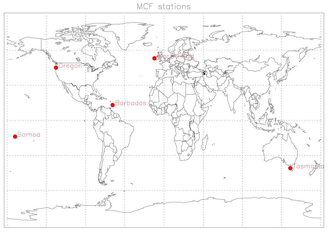
ALE/GAGE measurements of MCF have been taken from 1978. Five measurement stations are located in the 'clean' remote regions. Whenever applicable, pollution events have been omitted from the data. The asterisks in the following plots denote monthly averages. Bars denote standard deviations. It can be observed that the NH stations show considerably more variability due to the proximity of the sources. In the tropics, variability is mainly caused by convection.
Mace Head (53N, 11W) |
|
In order to simulate the MCF concentrations, we need to run the model for a longer period. The lifetime of MCF is 4-5 years, so we need a spin up time of at least 4 years. The model is initialized by concentrations of 40 ppt (parts per trillion) in 1975 and is run from then. First we set the reaction rate to
- k = 5e-12*exp(-1550/T) cm3molecules-1s-1
to see if this is a reasonable choice. The input file mcf.in requests a five year MOGUNTIA run and specifies the emissions (see EMISSION DISTRIBUTION) and chemical destruction by OH with the rate stated before.
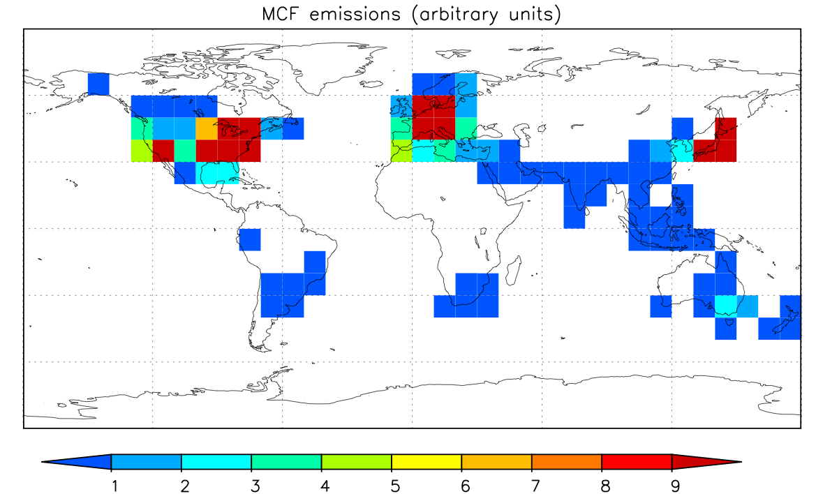
Figure 1: MCF emission distribution.
- run MOGUNTIA with the input file mcf.in (about fourty seconds)
- Discuss the simulated seasonal cycle.
- Discuss the latitudinal gradient.
- Should the rate be higher/lower?
Now, adjust the MCF + OH reaction rate and rerun:
- Adjust the rate in mcf.in
- Rerun MOGUNTIA up to 1980
- Again, check the 1980 concentrations.
- Check the seasonal cycle and the latitudinal gradient
Once you are confident that the rate is about correct, a longer period can be simulated:
- Adjust the END_DATE to 19940101 in mcf.in
- Rerun MOGUNTIA up to 1994 (ignore the message at the end of the run by pressing <Enter>)
- Compare simulation and measurements
- Discuss differences in variability, seasonal cycle, and trend.
- Estimate the uncertainty in the rate constant. This uncertainty can also be interpreted as uncertainty in the OH fields.
- Is MCF a good tracer to constrain the OH fields (see introduction)?
Exercise 8: More recent MCF measurements
The simulation of MCF with MOGUNTIA seems to work reasonable for the period 1978-1994. A rigorous test for the estimated rate of removal (k OH) is the application of this removal to more recent measurements. Is the removal rate estimated for 1978-1994 applicable for 1990-2009? In this period, we are observing a decaying burden of MCF, due to strongly reduced emissions
In order to set up a simualtion for the later period we need:
- A suitable start concentration.
- The optimized rate constant from the previous exercise.
- Yearly emissions for the 1990-2009 period.
- Measurements to check the consistency of the simulation.
Measurements from the GAGE (red) and AGAGE (green) network can be found below.
Mace Head (53N, 11W) |
|
- Open the MOGUNTIA input file in an editor mcf_new.in.
- Fill in the reaction rate that is consistent with previous exercise (1975-1993).
- Estimate a suitable start concentration in 1990 from the plots above. Note that the concentrations in 1990 are much higher on the NH, some some compromise is needed.
- Perform a simulation. Tip: to find a suitable start concentration, start with a run-time that is initially shorter (1990-1992).
Questions
- What do you observe for the seasonal cycle?
- What do you observe for the north-south gradient in MCF?
- How do these features compare to the observations?
- How do the end concentrations match with the observed concentration?
- What is your conclusion about the suitability of the rate constant derived for 1978-1994?
- Did the global OH concentration change much from the 1980s to the recent period?
Extra
In reality we have to account for the uptake of MCF by the oceans and removal in the stratosphere. In this extra exercise we will investigate the impact of these additional sinks on the simulations
- The time scale for removal by the ocean is estimated as about 80 years. The time scale for stratospheric removal as 45 years. Calculate the overall time scale for the combined processes
- Select the LIFE_TIME such that the sink accounts for these removal processes
- Redo the first exercise and re-estimate the removal rate (k).
- Is this k lower or higher? Why?
- Also repeat the second simulation, now with the newly estimated k and the estimated lifetime. Does the situation improve?