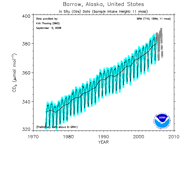
Figure 1: CO2 concentration (ppm or micro-mol/mol) measured at Barrow (Alaska) between 1974 and 2006.
Simulate the growth in atmospheric mixing ratios of CO2 as a result of fossil fuel emissions. Compare the simulated growth rate to observed growth rates and estimate what fraction of the emitted CO2 stays in the atmosphere.
The atmospheric concentration of CO2 has been increasing from about 330 ppm in 1974 to about 380 ppm in 2006 (see figure 1).There is little doubt that the CO2 emissions that are related to fossil fuel use are responsible for the increase in atmospheric CO2 concentrations. But what would be the increase in atmospheric concentrations if all the CO2 would remain in the atmosphere? And what is the gradient between the Northern Hemisphere (most emissions) and the Southern hemisphere (less emissions). To test this, CO2 will be added as an non-reactive tracer with only fossil fuel emissions. Other processes, such as uptake by the biosphere, oceans, and emission as a result of biomass burning, are ignored.
In order to compare to model to a real atmosphere, measurements taken by NOAA/CMD will be used. The link is given below. Also, the Carbon Dioxide Information Analysis Center provides estimates of world-wide CO2 emissions. The web-addresses are used throughout the exercises.
Table 1: relevant web-addresses for the exercises
| CO2 measurements made by NOAA/CMD | http://www.esrl.noaa.gov/gmd/dv/iadv/ |
| Estimates of fossil emissions CO2 | http://cdiac.ornl.gov/trends/emis/overview_2006.html |
In the following exercises, it will be attempted to:
First, the MOGUNTIA model has to initialised. A prelimanary input file fossil.in is provided as a starting point. Note that the MOLMASS is defined as 12, since all data are normally given in Millions of Tonnes (1 pG = 1000 Million Tonnes) of carbon. Note also that the CO2 emission distribution is read from a file. Logically, highest emissions are found over industrialised and densily populated areas.
Initially, the model will be run for four years (2000, 2001, 2002, 2003) with the CDIAC fossil fuel emissions.
In order to get a first estimate of the CO2 that is taken up by the oceans and biosphere, try to reduce the emissions and rerun the model to get a better correspondance to observations.
In order to estimate the long-term average uptake of CO2 in a more sophisticated way, the following diagram is used:
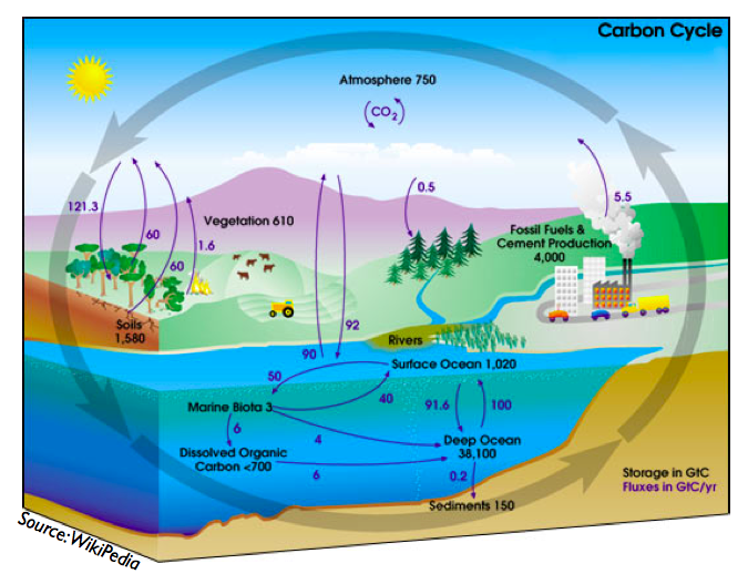
Figure 2: Diagram showing the estimated budget for CO2. Blue numbers indicate fluxes in GtC/yr and black numbers indate reservoirs in GtC. 1 GtC corresponds to 10 to the power 12th gram, or 1 Pg.
From the net uptake of CO2, e.g. to the oceans, a lifetime can be calculated by dividing the atmospheric burden by the net-uptake. The task is now to test these numbers in MOGUNTIA. For that reason, the input file is modified in the following way:
Address the following issues
Repeat the calculations for: