Flattening Images with Step Edges and Atomic or Molecular Resolution
This example continues with the Python shell session from the previous topic Flattening Images with Step Edges. In this example you learn how to flatten an image with step edges which does have molecular or atomic resolution. Locating step edges on images with clear atomic contrast is difficult because the step finding routine is looking for high gradients in the image, but each atom has a steep gradient surrounding it. For flattening the following functions are suitable:
flatten_poly_xy()(only first order and without a mask)
For locating regions in an image:
For locating step edges in an image:
Tutorial Example
Open the demo image image_with_step_edge_and_atoms.dat:
>>> im = spiepy.demo.load_demo_file(demos[2])
The variable im is the original demo image. Before trying to locate the step
edge, remove the tilt on the surface as much as possible. This improves the
contrast of the step. Only first order polynomial planes should be used as
higher order polynomials will try to fit the step. Either the function
flatten_poly_xy() or flatten_xy() can be used to do this. Now
flatten the image with the function flatten_xy():
>>> im_flat, _ = spiepy.flatten_xy(im)
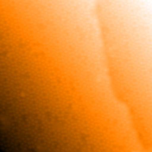
The variable im_flat contains the flattened image, it is the input image minus fitted plane. im is not overwritten, the data will be flattened again later and it is best to avoid cumulative flattening where possible. The flattened image looks like:

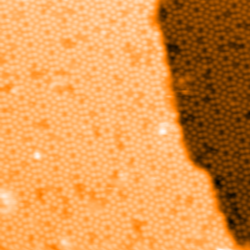
While the contrast of the step edge is quite strong it is clear that there is a
strong change in contrast between each atom and the space around it. The
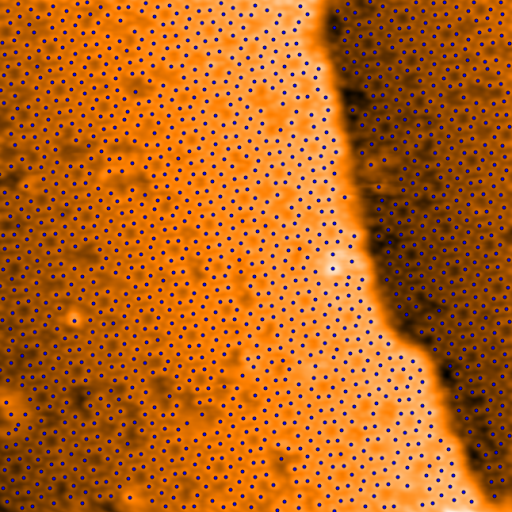
contrast of the atoms must be removed. The function locate_regions() will
locate the positions of the atoms and will create an image from the input image
with adjusted contrast. Make it so:
>>> regions, peaks = spiepy.locate_regions(im_flat)
Showing now the flattened images with atoms marked and with adjusted contrast.
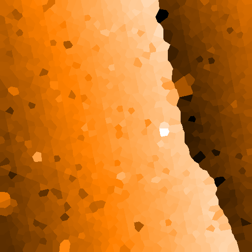
The contrast of the step is now very clear in the image. Find the step edge in
regions with the function locate_steps():
>>> mask = spiepy.locate_steps(regions, 5)
Showing now the flattened image with the mask (step edge).
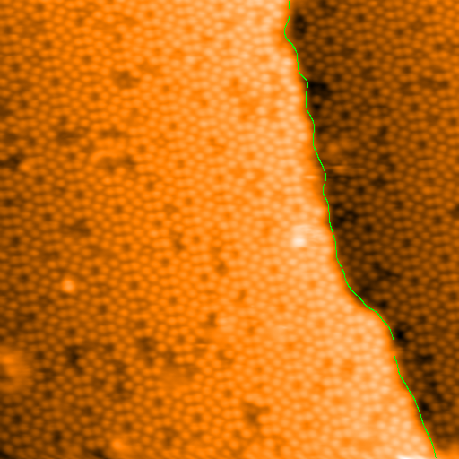
Once the step edges has been successfully located, the image can be
re-flattened with the function flatten_xy(). Flatten the original image
again using the keyword argument mask and the variable mask:
>>> im_final, _ = spiepy.flatten_xy(im, mask)
It is clear that each terrace is now free of its gradient. A final check which can be applied is to plot a histogram of the pixel heights for the images im_flat and im_final.
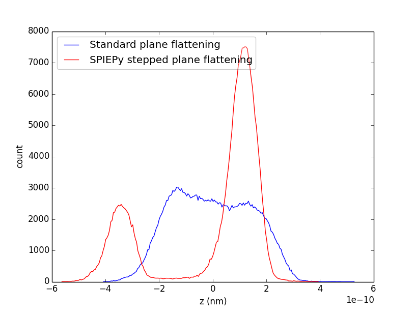
The two terraces are clearly separated!